Example: Head Controlled Well

This example demonstrates how pymf6 can be used to control the rate of an extraction well so that the well water level does fall below under a given water level.

Using a simple model

The model was created with flopy with a script in pymf6-tools. You may use any GUI tool such as ModelMuse to create such a model. This is not specific to pymf6 but helps to better understand the problem. You may skip ahead to the section with use of pymf6.

make_input(model_data)

Geometry

The model has 1, layer, 10 rows, and 10 columns with a size of 1 m in all dimensions:

name	value
nrow	10
ncol	10
nlay	1
delr	1.0
delc	1.0
top	1.0
botm	0.0

It has two constant head boundary conditions in the corners and a well in the middle:

show_bcs(model_path=model_path, name=name, bc_names=('wel', 'chd'));

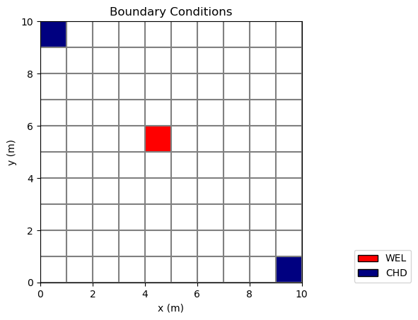
There are 4 stress periods. The first is steady state to get consistent starting conditions. The next three stress periods are transient:

BEGIN options
  TIME_UNITS  days
END options

BEGIN dimensions
  NPER  4
END dimensions

BEGIN perioddata
       1.00000000  1       1.00000000
      10.00000000  120       1.00000000
      10.00000000  120       1.00000000
      10.00000000  120       1.00000000
END perioddata

There is no pumping in the first, steady state stress period. The pumping rate varies between the following, transient, stress periods:

BEGIN options
END options

BEGIN dimensions
  MAXBOUND  1
END dimensions

BEGIN period  2
  1 5 5 -5.00000000E-02
END period  2

BEGIN period  3
  1 5 5 -5.00000000E-01
END period  3

BEGIN period  4
  1 5 5 -5.00000000E-02
END period  4

Looking at the model results

After running the model, we can look at the results. This function visualizes the head at the end of the last time step:

show_heads(model_path=model_path, name=name, title='', show_wells=True);

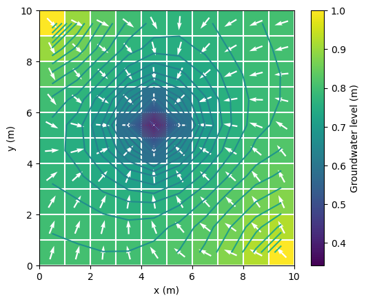
The well is roughly in the middle of the model. The yellow cells have a constant water level and “feed” the model. The well causes a cone of depression:

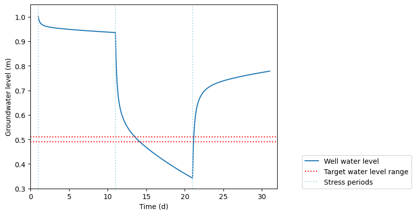
The four stress periods are indicated by the blue dotted vertical lines. The first period, that is steady state, has only one time step. Periods two to four are transient from day 1 to 11, 11 to 21, and 21 to 31 with different extraction rate. The well water level reflects the pumping. Period three has the full rate and periods two and four have only a tenth of the rate. The two dotted read horizontal lines show the desired mininmum well water level of 0.5 m with a corridor of 0.01 m.

Working with pymf6

Now, we will use pymf6. The objective is the avoid a drop of the groundwater level at the well below a given limit.

wel_coords = model_data['wells']['wel_out']['coords']

Creating the input files:

make_model.make_input(
    pymf6_model_data
)

We run the model with pymf6. We need to import the class MF6:

from pymf6.mf6 import MF6

We define variables, holding the values for the target water level and the tolerance that define the limits of allowed corridor:

tolerance = 0.01
head_limit = 0.5
upper_limit = head_limit + tolerance
lower_limit = head_limit - tolerance

We creat and instance of the MF6:

MF6?

Init signature:
MF6(
    sim_path,
    dll_path=None,
    use_modflow_api=True,
    advance_first_step=True,
    verbose=False,
    new_step_only=False,
    do_solution_loop=True,
    _develop=False,
)
Docstring:     
Wrapper around XmiWrapper and modflowapi.

`advance_first_step = True` progresses to the first model step with
model time > 0. This is needed to access any internal values of BCs.
File:           ~/Dev/pymf6/src/pymf6/mf6.py
Type:           type
Subclasses:     

mf6 = MF6(model_path)

There are only flow models:

mf6.models.keys()

dict_keys(['gwf6'])

Get the flow models:

gwf_models = mf6.models['gwf6']

There is onyl one flow model:

gwf_models.keys()

dict_keys(['headconwell'])

We get a reference to this model:

gwf = gwf_models['headconwell']

These are the available packages:

gwf.packages

	description	is_mutable
name
dis	DIS Package: DIS	False
hfb	HFB Package: HFB	True
csub	CSUB Package: CSUB	True
mywell	WEL Package: MYWELL	True
mvr	MVR Package: MVR	True
ic	IC Package: IC	False
vsc	VSC Package: VSC	True
chd_0	CHD Package: CHD_0	True
buy	BUY Package: BUY	True
gnc	GNC Package: GNC	True
sto	STO Package: STO	False
npf	NPF Package: NPF	False

Model packages

Packages can be accessed via model.packages.package_name. If package_name is not a valid Python identifier, access with pandas logic model.packages.loc['package_name']. Packages that are mutable (is_mutable is True) can be converted in a mutable boundary condition with .as_mutable_bc().

The well boundary condition is mutable. But, since no well is defined in the first, steady state, period, it cannot be turned into a mutable boundary condition:

gwf.packages.mywell.as_mutable_bc()

ValueError: No values yet.
Boundary condition MYWELL does not have any values for current stress periods.
Advance to a stress period with values and call this function again.

We get a hold of the model loop:

loop = mf6.model_loop()

and fast-forward to start of second time stress period:

for model_step in loop:
    if gwf.kper > 0:
        break

Now, we can create a mutable boundary condition:

mywell = gwf.packages.mywell.as_mutable_bc()

The well is avilable:

mywell

	nodelist	q
0	(0, 4, 4)	-0.05

We can also acces the value of the pumping:

mywell.q[0]

np.float64(-0.05)

The well coordinates are also accessible:

mywell.nodelist[0]

(np.int64(0), np.int64(4), np.int64(4))

Using this coordinate, we can get the current groundwater level in well cell:

gwf.X[mywell.nodelist[0]]

np.float64(1.0)

Let’s create a nicer name for the coordinates

mywell_coords = mywell.nodelist[0]

We define a helper variable been_below, that will be helpful to remember if well water level was below the defined limit.

been_below = False

We use dictionary to store the modified pumping rates over time:

mywell_q = {'step': [], 'q': []}

Now we loop the timesteps. We influence the pumping only in the third stress period, i.e. when gwf.kper is 2:

for model in loop:
    if gwf.kper == 2:
        mywell_head = gwf.X[mywell_coords]
        if mywell_head <= lower_limit:
            been_below = True
            mywell.q *= 0.9
        elif been_below and mywell_head >= upper_limit:
            mywell.q *= 1.1
        mywell_q['step'].append(gwf.kstp)
        mywell_q['q'].append(mywell.q[0])

If the groundwater level in the well cell is below the given limit (minus the tolerance), we set been_below to True and reduce the pumping rate by 10%. If the cell water level was below the level before, i.e. if been_below is True, and the water level is above the given limit (plus the tolerance), we increase the pumping rate by 10%.

Looking at the results

Now the water level stays just around 0.5 m:

show_my_well_head(model_data=pymf6_model_data);

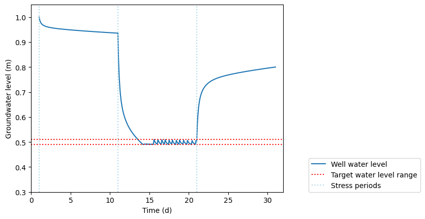
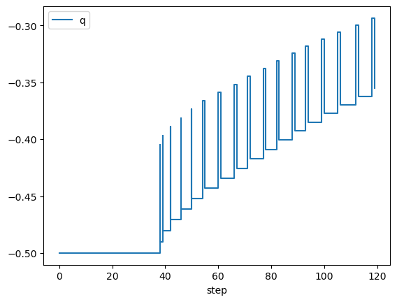
The water level oscillates tightly in the corridor between lower and upper limit. The pumping is modified frequently:

import pandas as pd

pd.DataFrame(mywell_q).plot(x='step');

Further steps

The control of the pumping rate is not very realistic. These a few things that can be done with a few lines of Python:

• Make tolerance corridor wider

• Use discrete pumping rate level instead of 10% changes