Example: Head Controlled Well

This example demonstrates how pymf6 can be used to control the rate of an extraction well so that the well water level does fall below under a given water level.

Setting up a model with flopy

First, we create a simple model with flopy. You may use any GUI tool such as ModelMuse to create such a model. This is not specific to pymf6 but helps to better understand the problem. You may skip ahead to the section with use of pymf6.

Creating the input data

First, we import a few need libraries:

"""Create, run, and postprocess a MODFLOW 6 model with flopy.
"""

import flopy
from flopy.utils.postprocessing import get_specific_discharge
from matplotlib import pyplot as plt
import numpy as np

The function make_input creates our model with help pf flopy:

def _make_wel_stress_period(gwf, wel_q, wel_coords):
    """Create stress period data for the wel package."""
    period = flopy.mf6.ModflowGwfwel.stress_period_data.empty(
        gwf,
        maxbound=1,
    )
    period[0][0] = (wel_coords, wel_q)
    return period


def make_input(
    wel_q,
    wel_coords,
    model_path,
    name,
    exe_name='mf6',
    verbosity_level=0):
    """Create MODFLOW 6 input"""
    sim = flopy.mf6.MFSimulation(
        sim_name=name,
        sim_ws=model_path,
        exe_name=exe_name,
        verbosity_level=verbosity_level,
    )
    times = (10.0, 120, 1.0)
    tdis_rc = [(1.0, 1, 1.0), times, times, times]
    flopy.mf6.ModflowTdis(
        sim, pname="tdis",
        time_units="DAYS",
        nper=4,
        perioddata=tdis_rc,
    )
    flopy.mf6.ModflowIms(sim)
    gwf = flopy.mf6.ModflowGwf(sim, modelname=name, save_flows=True)
    flopy.mf6.ModflowGwfdis(gwf, nrow=10, ncol=10)
    flopy.mf6.ModflowGwfic(gwf)
    flopy.mf6.ModflowGwfnpf(
        gwf,
        save_flows=True,
        save_specific_discharge=True,
        icelltype=[0],
        k=[0.5],
        k33=[0.1],
    )
    sy = flopy.mf6.ModflowGwfsto.sy.empty(
        gwf,
        default_value=0.2
    )
    ss = flopy.mf6.ModflowGwfsto.ss.empty(
        gwf, default_value=0.000001
    )
    flopy.mf6.ModflowGwfsto(
        gwf,
        pname="sto",
        save_flows=True,
        save_specific_discharge=True,
        iconvert=1,
        ss=ss,
        sy=sy,
        transient={0: True},
        )

    stress_period_data = {
        1: _make_wel_stress_period(gwf, wel_q / 10, wel_coords)[0],
        2: _make_wel_stress_period(gwf, wel_q, wel_coords)[0],
        3: _make_wel_stress_period(gwf, wel_q / 10, wel_coords)[0]
    }
    flopy.mf6.ModflowGwfwel(
        gwf,
        stress_period_data=stress_period_data,
    )
    flopy.mf6.ModflowGwfchd(
        gwf,
        stress_period_data=[
            [(0, 0, 0), 1.],
            [(0, 9, 9), 1.]],
    )
    budget_file = name + '.bud'
    head_file = name + '.hds'
    flopy.mf6.ModflowGwfoc(
        gwf,
        budget_filerecord=budget_file,
        head_filerecord=head_file,
        saverecord=[('HEAD', 'ALL'), ('BUDGET', 'ALL')])
    sim.write_simulation()

We specify some data for the model:

model_path=r'models\mf6'
name='headconwell'
wel_coords=(0, 4, 4)
wel_q = -0.5

and create the input files.

make_input(
    wel_q=wel_q,
    wel_coords=wel_coords,
    model_path=model_path,
    name=name
)

Running the model

The function get_simulation retrieves a flopy simulation object:

def get_simulation(model_path, exe_name='mf6', verbosity_level=0):
    """Get simulation for a model."""
    sim = flopy.mf6.MFSimulation.load(
        sim_ws=model_path,
        exe_name=exe_name,
        verbosity_level=verbosity_level,
    )
    return sim

This function runs the model:

def run_simulation(model_path, verbosity_level=0):
    """Run a MODFLOW 6 model"""
    sim = get_simulation(
        model_path,
        verbosity_level=verbosity_level)
    sim.run_simulation()

We run the simulation:

run_simulation(model_path=model_path)

There is visible output from MODFLOW 6. Setting the verbosity_level to 1 or higher in run_simulation will show the simulations steps.

Looking at the model results

Let’s look at the model results. This function visualizes the head at the end of the last time step:

def show_heads(model_path, name):
    """Plot calculated heads along with flow vector."""
    sim = get_simulation(model_path, name)
    gwf = sim.get_model(name)

    head = gwf.output.head().get_data()
    bud = gwf.output.budget()

    spdis = bud.get_data(text='DATA-SPDIS')[-1]
    qx, qy, _ = get_specific_discharge(spdis, gwf)
    pmv = flopy.plot.PlotMapView(gwf)
    pmv.plot_array(head)
    pmv.plot_grid(colors='white')
    pmv.contour_array(
        head,
        levels=np.arange(0.2, 1.0, 0.02),
    )
    pmv.plot_vector(qx, qy, normalize=True, color="white")

We look at the heads:

show_heads(model_path=model_path, name=name)

The well is roughly in the middle of the model. The yellow cells have a constant water level and “feed” the model. The well causes a cone of depression.

This function shows the head the well location over time:

def show_well_head(model_path, name, wel_coords):
    """Plot head at well over time."""
    sim = get_simulation(model_path, name)
    gwf = sim.get_model(name)
    heads = gwf.output.head().get_ts(wel_coords)
    _, ax = plt.subplots()
    ax.plot(heads[:, 0], heads[:, 1])

This is the head at the well over time:

show_well_head(model_path=model_path, name=name, wel_coords=wel_coords)

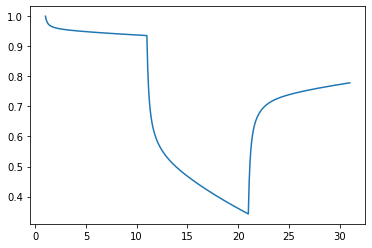
There are four stress periods. The first period is steady state. Periods two to four a transient with different extraction rate. Period three has the full rate and periods two and four have only a tenth of the rate. See generation of the input files for details.

Working with pymf6

Finally, we will use pymf6. The objective is the avoid a drop of the water level at the well below a given limit.

Creating new input files

We generate the input files again. There are no differences in the files to the model above. The only difference is the model directory:

model_path=r'models\pymf6'

Creating the input files:

make_input(
    wel_q=wel_q,
    wel_coords=wel_coords,
    model_path=model_path,
    name=name
)

Run the model with pymf6

Now run the model with pymf6:

from pymf6.mf6 import MF6

def run_model(nam_file):
    mf6 = MF6(nam_file=nam_file)
    head = mf6.vars['SLN_1/X']
    wel_index = 44
    tolerance = 0.01
    head_limit = 0.5
    upper_limit = head_limit + tolerance
    lower_limit = head_limit - tolerance
    wel = mf6.vars['HEADCONWELL/WEL_0/BOUND']
    been_below = False
    for step in mf6.steps():
        if step < 21:
            if head[wel_index] <= upper_limit:
                wel[:] = wel[:] * 0.9
                been_below = True
            elif been_below and head[wel_index] >= upper_limit:
                wel[:] = wel[:] * 1.1

The class MF6 provides the functionality of pymf6. The dictionary mf6.vars provides all MODFLOW 6 variables. The head has the name SLN_1/X and the values of the boundary condition WEL is HEADCONWELL/WEL_0/BOUND. The name will change depending on model name and the chosen name for the boundary condition.

mf6.steps() provides a generator that allows to iterate over all MODFLOW 6 time steps. step is the current time step in the unit specified in the input files, here DAYS. We don’t want influence the last, which starts at day 21. We adjust the extraction rate by reducing o increasing the rate by 10%, if the water level at the well, found at index 44, is not within the upper and lower limit.

Running the model:

run_model(r'models/pymf6/mfsim.nam')

Looking at the results

Now the water level stays just around 0.5:

show_well_head(model_path=model_path, name=name, wel_coords=wel_coords)

There is some oscillation in the water level. These can be reduced by adding more time steps in the TDIS package.