%load_ext jbmagics
Problem adaption
Create a sinusoidal groundwater level
from flopy.mbase import run_model

import matplotlib.pyplot as plt
import numpy as np

from pymf6tools.custom_print import CustomPrint

from helpers import make_model_input, get_flux, plot
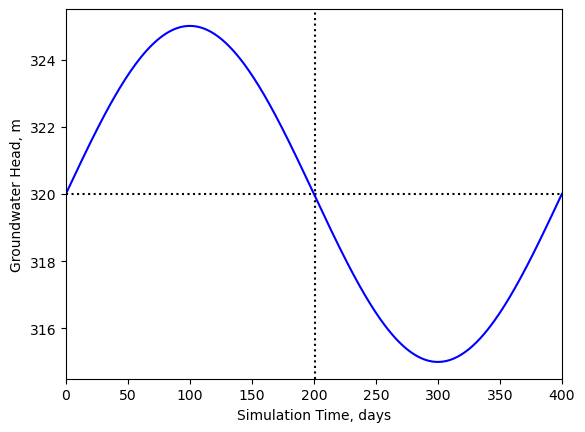
The water level with oscillate between 320 and 325 meters:
h_mean, h_min, h_max = 320.0, 315.0, 325.0
amplitude = (h_min - h_max) / 2.0
Using 401 discrete time steps, we get this sinus curve of the groundwater level:
ntimesteps = 401
ihalf = int(ntimesteps / 2) + 1
x = np.linspace(-np.pi, np.pi, ntimesteps)
chd_head = amplitude * np.sin(x) + h_mean
plt.axhline(h_mean, color="black", ls=":")
ax = plt.gca()
ax.axvline(ihalf, color="black", ls=":")
ax.plot(chd_head, color="blue")
ax.set_xlabel("Simulation Time, days")
ax.set_ylabel("Groundwater Head, m")
ax.set_xlim(0, 400);
Creating a model
Using flopy, we create a simple MODFLOW model.
It is has 2 layers, 1 row, and 1 column.
There are two boundary conditions,
(a) constant head will in the lower layer (layer 2) and
(b) the river boundary cell in the upper layer model (layer 1):
%%include helpers.py
end_at = "import matplotlib"
import_module = True
"""Helpers to create a MF6 model."""

from pathlib import Path

import flopy.mf6 as fp
import matplotlib.pyplot as plt
%%include helpers.py
start_at = "def make_model_input"
end_at = "return sim"
import_module = True
def make_model_input(name, chd_head, h_mean):
    """Create model input."""
    ws = Path(name)
    sim = fp.MFSimulation(sim_name=name, sim_ws=ws, memory_print_option='all')
    pd = [(1, 1, 1.0)] * chd_head.shape[0]
    tdis = fp.ModflowTdis(sim, nper=len(pd), perioddata=pd)
    ims = fp.ModflowIms(
        sim, complexity='simple', outer_dvclose=1e-6, inner_dvclose=1e-6
    )
    gwf = fp.ModflowGwf(
        sim,
        modelname=name,
        print_input=True,
        save_flows=True,
    )
    dis = fp.ModflowGwfdis(
        gwf,
        nlay=2,
        nrow=1,
        ncol=1,
        delr=1.0,
        delc=1.0,
        top=360,
        botm=[220, 200],
    )
    npf = fp.ModflowGwfnpf(
        gwf,
        k=50.0,
        k33=10.0,
    )
    ic = fp.ModflowGwfic(gwf, strt=chd_head[0])
    condref = 1.0
    spd = [((0, 0, 0), h_mean, condref, 319.0)]
    riv = fp.ModflowGwfriv(
        gwf, stress_period_data=spd, pname='RIVER', print_flows=True
    )
    spd = {idx: [((1, 0, 0), h)] for idx, h in enumerate(chd_head)}
    chd = fp.ModflowGwfchd(gwf, stress_period_data=spd, print_flows=True)
    oc = fp.ModflowGwfoc(
        gwf,
        head_filerecord=f'{name}.hds',
        budget_filerecord=f'{name}.cbc',
        printrecord=[('budget', 'all')],
        saverecord=[('head', 'all'), ('budget', 'all')],
    )
    sim.write_simulation()
    return sim
Create the input files:
name = 'rivercond'
sim = make_model_input(name, chd_head, h_mean)
writing simulation...
  writing simulation name file...
  writing simulation tdis package...
  writing solution package ims_-1...
  writing model rivercond...
    writing model name file...
    writing package dis...
    writing package npf...
    writing package ic...
    writing package river...
INFORMATION: maxbound in ('gwf6', 'riv', 'dimensions') changed to 1 based on size of stress_period_data
    writing package chd_0...
INFORMATION: maxbound in ('gwf6', 'chd', 'dimensions') changed to 1 based on size of stress_period_data
    writing package oc...
and run the model:
Running the model
sim.run_simulation(custom_print=CustomPrint(show_each_stress_period=False));
                                   MODFLOW 6
                U.S. GEOLOGICAL SURVEY MODULAR HYDROLOGIC MODEL
                            VERSION 6.6.0 12/19/2024

        MODFLOW 6 compiled Dec 19 2024 21:26:44 with GCC version 13.3.0

This software has been approved for release by the U.S. Geological
Survey (USGS). Although the software has been subjected to rigorous
review, the USGS reserves the right to update the software as needed
pursuant to further analysis and review. No warranty, expressed or
implied, is made by the USGS or the U.S. Government as to the
functionality of the software and related material nor shall the
fact of release constitute any such warranty. Furthermore, the
software is released on condition that neither the USGS nor the U.S.
Government shall be held liable for any damages resulting from its
authorized or unauthorized use. Also refer to the USGS Water
Resources Software User Rights Notice for complete use, copyright,
and distribution information.


 MODFLOW runs in SEQUENTIAL mode

 Run start date and time (yyyy/mm/dd hh:mm:ss): 2025/01/05  8:01:10

 Writing simulation list file: mfsim.lst
 Using Simulation name file: mfsim.nam

    Solving:  Stress period:   401    Time step:     1

 Run end date and time (yyyy/mm/dd hh:mm:ss): 2025/01/05  8:01:10
 Elapsed run time:  0.082 Seconds

 Normal termination of simulation.
Looking at the results
We retrieve the flux from the river boundary cell:
%%include helpers.py
start_at = "def get_flux"
end_at = "return"
import_module = True
def get_flux(sim, name):
    """Get flux data model output."""
    gwf = sim.get_model(name)
    bud = gwf.output.budget()
    riv = bud.get_data(text='RIV')
    flux = [float(entry['q'][0]) for entry in riv]
    return flux
flux = get_flux(sim, name)
and plot its values over time:
%%include helpers.py
start_at = "def plot"
end_at = "return"
import_module = True
def plot(flux, vmin=-0.6, vmax=0.6, cell_name='river'):
    """Plot the river flux."""
    fig, ax = plt.subplots(
        nrows=1,
        ncols=1,
        layout='constrained',
        figsize=(4.5, 5),
    )
    ax.set_title(f'Flux in {cell_name} cell')
    ax.set_xlim(0, 400.0)
    ax.set_ylim(vmin, vmax)
    ax.set_xlabel('Simulation time, days')
    ax.set_ylabel('Flow tate, m$^3$/d')
    ax.axhline(0, lw=0.5, ls='-.', color='black')
    ax.plot(
        flux,
        color='black',
        lw=1.0,
        label='River flux',
    )
    ax.legend()
    return ax
plot(flux);
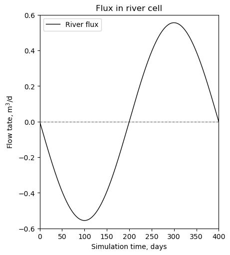
The flux shows the same pattern as the groundwater level. The river conductance is constant.